


Multisampling is a well-understood technique used in computer graphics that enables applications to efficiently reduce geometry aliasing, yet not everybody is familiar with the entire toolset offered by modern GPU hardware to control multisampling behavior. In this article we present the behavior of basic multisampling and explore a set of controls that enable us to tune performance/quality trade-offs and open doors for more advanced rendering techniques.
While it’s quite common nowadays for renderers to use other, lower cost and often less intrusive techniques to reduce screen-space aliasing like temporal anti-aliasing or various morphological techniques, multisampling remains prevalent as a standard go-to technique to perform anti-aliasing, is often used in conjunction with the aforementioned alternatives, and sometimes (ab)used to aid more complex rendering algorithms like checkerboard rendering to achieve better perceived resolution, quality, and/or performance. Hence familiarity with the behavior and configuration parameters available in modern multisampling hardware implementations comes handy in a wide set of rendering problems.
Naive Supersampling
In general, any sort of screen-space aliasing is the result of the very nature of evaluating rendering functions at discrete units (typically per-pixel, at pixel centers) hence producing noticeable under-sampling induced artifacts.
Supersampling improves this by increasing the sampling resolution of the entire rendering pipeline. The simplest way to implement supersampling is to render at a higher resolution than the final target (e.g. twice the width and height to achieve 4x supersampling) and then downsampling the produced image to the target resolution, usually with a simple box filter. This downsampling process is called a resolve operation.

From a terminology perspective this leads us to the notion of sample whereas we refer to the collection of values in the supersampled image contributing to a particular value in the final target image as pixels, and we call the individual values within those collections as the samples of the pixel.
Obviously, supersampling doesn’t completely eliminate aliasing, really nothing can in a discrete processing pipeline, however it can significantly reduce its effect. The quality improvement is roughly proportional to the number of samples evaluated per pixel, i.e. the ratio of the resolution at which the rendering pipeline was evaluated and the resolution at which the results are displayed. The main problem with naive supersampling is that the performance and memory usage cost is also increased by the same ratio.
Basic Multisampling
Multisampling is essentially a performance optimization to supersampling where certain operations within the graphics pipeline that don’t have significant (or sometimes any) effect on aliasing are allowed to operate at a reduced rate. This enables multisampling to achieve better overall performance-to-quality ratio than naive supersampling.
In order to understand where we can reduce processing rate, let’s look at the relevant graphics pipeline stages and resources:

Note: fragments may correspond to whole pixels or to individual samples within a pixel.
Clearly, rasterization, depth/stencil testing, color buffer operations, and generally all fixed-function per-fragment operations, have to happen at full rate in order to actually produce an effectively higher resolution image with multiple samples per pixel that can be later resolved to the display resolution. This also implies that our depth/stencil buffer and color buffer(s) also need to be able to store such a higher resolution image, or, in practice, multiple samples per pixel. We call these multisampled images (or textures) and their effective resolution is specified through a width, height, and number of samples (with the addition of a depth and/or layer count parameter for 3D/layered textures, if applicable).
We can note here though that evaluating the fragment shader for each sample of a pixel separately doesn’t seem to provide much benefit as it’s a reasonable assumption that evaluating color values for each sample separately and then averaging those when resolving the multisampled image(s) should result in the same color value that we get if we only evaluate a single color value per pixel. Obviously, this ignores certain details that make this assumption incorrect in general, as we will see later, often there’s little to no perceived difference between the two.
Multisampling takes advantage of this by executing only a single fragment shader invocation for each pixel a primitive overlaps with, no matter how many samples within that pixel the primitive actually covers. As fragment shading is typically the most expensive stage in the graphics pipeline back-end, this can save significant processing time compared to supersampling. In cases where the additional bandwidth cost of multisampled color and depth/stencil buffers, and the additional load on the fixed-function stages responsible for rasterization, depth/stencil testing and color buffer operations don’t saturate the corresponding hardware resources, basic multisampling induces a relatively small overhead compared to single-sampled rendering, unlike supersampling.
Integrating basic multisampling into a renderer is quite straightforward as it requires little to no modifications aside from the additional resolve operation needed before presenting the final rendering. However, in practice, things get complicated when considering certain special cases discussed later, and as modern rendering workloads often involve passes rendering to intermediate framebuffers used for post-processing, shadow mapping, and other purposes, developers have to choose carefully which passes should they apply multisampling to.
Coverage
This is a new term that needs to be introduced in the context of multisampling. The coverage of a pixel with respect to a particular incoming primitive provides information about which samples within a pixel actually overlap the primitive in question. This coverage information is generally represented as a binary number called the coverage mask where the ith digit (bit) of the number contains 1 if the ith sample of the pixel is inside (is covered by) the primitive, and 0 otherwise. When a sample’s corresponding coverage mask bit is set, it’s often referred to as the sample being lit.
The coverage mask needs to be available across the post-rasterization graphics pipeline stages, as it affects their operation:
- The original coverage mask determined by rasterization (often called pre-depth coverage mask) needs to be available to depth/stencil testing to know which samples need to be tested
- Depth/stencil testing will set each bit of the coverage mask whose corresponding samples failed the test to
0, producing the post-depth coverage mask - Color buffer operations then use this post-depth coverage mask to limit writing the output color(s) of the fragment shader only for the samples whose corresponding bits are set in the mask
The pre-depth or post-depth coverage information can also be made available to the fragment shader as input, enabling more advanced rendering techniques, and the fragment shader may even output its own coverage mask which is then combined with the incoming coverage mask by subsequent pipeline stages using a bitwise AND operator (i.e. fragment shaders can’t add new covered samples, but can discard them), although there are some API extensions out there that also allow growing the set of covered samples using the fragment shader.

This notion of coverage will come handy when discussing more advanced multisampling features.
Additional Benefits
The processing scheme established by basic multisampling also allows for a set of techniques that provide performance and/or quality benefits that couldn’t be applied in a naive supersampling environment. In this section we will mention a few of those.
Bandwidth Optimizations
One thing to note about the effects of basic multisampling is that often the majority of samples within a pixel of the rendered image have the same color, as pixels covered entirely by the front-most primitive will get each of their samples’ color values coming from the same single fragment shader invocation.
Some GPUs take advantage of this through a novel scheme where color values of such pixels are only written to memory once, instead of being replicated for each sample of the pixel. This is achieved by decoupling the actual color value’s storage from the sample index it belongs to by introducing additional metadata that maps sample indices to storage locations. In such schemes, individual color values at separate storage locations within a pixel are often referred to as color fragments.
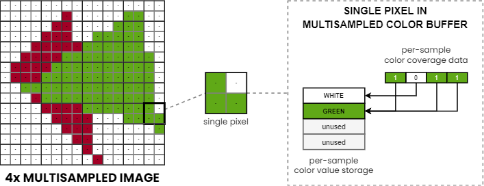
Note: illustration-only as support, representation, behavior, and the flexibility of mapping between samples and color fragments depends on the hardware implementation.
This provides us with a lossless color image compression scheme that is specifically tailored to reduce the bandwidth requirements of multisampled rendering, further reducing the performance gap compared to conventional single-sampled rendering.
For depth/stencil data the usual compression schemes work just as well in case of multisampling with a few caveats, as explained later.
Some GPUs go even further. In particular, as we’ve seen in our previous article, TBR GPUs can avoid storing multisampled data in off-chip memory altogether by performing multisampled rendering entirely on-chip and performing the resolve as part of the tile store operation responsible for committing on-chip result to RAM. This approach completely eliminates the additional external bandwidth costs of multisampling.
Sample Locations
Both single-sampled rendering and naive supersampling (implemented by doing single-sampled rendering at a higher resolution) evaluate per-fragment operations across a regular grid of sample points dictated by the center location of each pixel. Multisampling introduces additional flexibility here by not requiring the locations of samples within a pixel to form a uniform axis-aligned grid. In fact, hardware implementations historically used special empirically established sample location patterns that increase the perceived quality of anti-aliasing by breaking the uniform grid and resulting aliasing patterns.
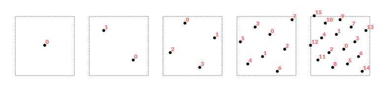
Nowadays, GPUs allow the application developer to specify the locations of samples within every 2×2 groups of pixels (quad) enabling further customization of multisampling behavior. This also opens the door for more advanced tricks where the sample locations are altered across subsequent frames and can be used as the basis for rendering techniques like checkerboard rendering or hybrid anti-aliasing algorithms combining multisampling and temporal anti-aliasing.
One thing to note here is that the location of the samples within a pixel has an effect on some of the compression schemes typically used for depth buffers. This means that multisampled depth buffer data can only be interpreted with respect to a particular set of sample locations. It’s thus no coincidence that graphics APIs like Vulkan rely on the specification of the sample locations used when performing any operations on a multisampled depth buffer that may require decompressing it, or otherwise interpreting its compressed contents.
Complications
As briefly mentioned earlier, even though basic multisampling can be easily deployed into existing rendering code, there are a whole set of cases that require special handling in order to produce the expected rendering results. Handling these cases appropriately can be fairly intrusive because it often involves the need for specialized shaders for the multisampling case. In this section we will take a look at a few of these special cases that all renderers employing multisampling should be aware of.
Texture Sampling
We talked about the shortcut multisampling takes compared to supersampling, whereas the fragment shader is evaluated only once, even if multiple samples within the pixel are covered by a primitive. Although it may not be immediately obvious, this shortcut can have significant effects on the final rendering when we look at the texture samples used by the fragment shader.
First, basic multisampling will sample textures only once per pixel and only at the center of the pixel (typically, at least), as texture samples are read by the fragment shader which itself is executed only once per pixel in the basic case. This already can have subtle side-effects due to the limited precision available in the various hardware components involved.
However, a more critical situation arises when the pixel center isn’t actually covered by the primitive for which fragment shading executes. This results in sampling the input textures at a location that is outside of the primitive, and can produce rendering artifacts where texture data belonging to another primitive can “leak” into the current one.
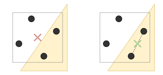
In order to avoid this, the coordinates at which textures are sampled may need to be altered to correspond to a screen-space location that lies inside the actual primitive’s footprint. Shading languages provide appropriate syntax to mark varyings (fragment shader inputs) to use centroid-based interpolation which guarantees that the corresponding values are interpolated at a location within the pixel that is actually covered by the primitive. Centroid-sampling is not without caveats though, as derivatives, and consequently the sampled LOD, may be affected by the unaligned sub-pixel sampling locations across the 2×2 pixel area (quad) used to calculate them.
Alpha Testing
Alpha testing has long ceased to exist as a dedicated fixed-function pipeline stage in GPUs (in most of them, at least) yet the term alpha testing stuck. What we really talk about here is the ability to cut out parts of a primitive based on some per-fragment data typically coming from a texture (often stored in the alpha channel). This is done by the fragment shader discarding certain sets of fragments.
As in the basic case of multisampling the fragment shader is only executed once per pixel, it follows that such cut-outs also happen per-pixel with a fragment shader designed for single-sampled rendering, hence the cut-out edges remain aliased, despite using multisampling.
Such shaders usually have to be altered to produce the expected results when used in conjunction with multisampling. There are multiple possible solutions to the problem with various levels of performance, quality, and intrusiveness.
The simplest solution is to just render such alpha-tested geometry separately, using supersampling. This guarantees correct rendering, however, it also eliminates the performance benefits of multisampling.
Another solution could be to manually loop over individual samples in the fragment shader (through the use of the input coverage mask), evaluate the condition of discarding for each, and adjust the output coverage mask according to the outcome of the test. This way we practically discard individual samples using the output coverage mask.
Clearly, this achieves identical results to supersampling, but in the process we also gave up most of the performance benefits of multisampling by having to execute at least part of the fragment shader per sample. This may or may not be any faster than supersampling, as on one hand we still kept the rest of the fragment shader code to execute per pixel instead of per sample, but on the other hand we made an otherwise parallelizable workload serial through the in-shader loop and, in general, made our fragment shader significantly more expensive.
A third option is to use a feature called alpha-to-coverage. This feature instructs the GPU to use the alpha channel of the first color output of the fragment shader to derive a corresponding coverage mask in some implementation dependent way where an alpha value of 0.0 results in a coverage mask with all bits set to 0, an alpha value of 1.0 results in a coverage mask with all bits set to 1, and for alpha values between those the produced coverage mask has a roughly proportiate number of bits set, potentially also applying some screen-space dithering. The derived coverage mask is then used as if it was the output coverage mask of the fragment shader. Using this feature enables a fairly non-intrusive way to keep the performance benefits of multisampling while still producing adequate anti-aliasing quality for alpha-tested geometry.
Advanced Multisampling
So far we only talked about the basic case of multisampling, but modern GPUs provide a wide set of parameters to control the behavior of it. Unfortunately, not all graphics APIs expose all of these. Truth be told, some of them are not universally or identically supported across all GPU vendors, while others are entirely vendor-specific, and at least many of them are actually exposed through cross-vendor and/or vendor-specific API extensions.
In order to have a structured look at the various configuration options, we have to introduce some new terminology…
In contrast to the single global sample count that is used in traditional supersampling and multisampling, we can define multiple different kinds of sample counts and collections of them used at different stages of the graphics pipeline:
- Rasterized samples (RSS) – the sample count at which rasterization and most per-fragment operations take place
- Depth/stencil samples (DSS) – the sample count at which depth/stencil testing takes place (the number of samples per pixel in the depth buffer)
- Shaded samples (SHS) – the number of fragment shader invocations per pixel
- Color coverage samples (CCS) – the sample count at which color buffer operations take place (the number of coverage samples per pixel in the color buffers)
- Color storage samples (CSS) – the number of unique color values per pixel the color buffers can store (the number of color storage samples per pixel in the color buffers)
The above terminology is sort of a combination of the terminology used across various GPU vendors. NVIDIA uses the term color samples to denote the actual samples with unique storage locations in the color buffers, and uses the term coverage samples for the samples which at least maintain color coverage information, while AMD sometimes uses the color samples term for the latter, and color storage samples or color fragments for the former. Little literature distinguishes between rasterized samples and (color) coverage samples, but for the purposes of the contents of this article it seemed appropriate.
The way various sets of samples are mapped to one another seem to vary across implementations to some extent where some may use fixed mapping while others may allow more dynamic mapping between certain types of sample counts. We will note some of these nuances when presenting the corresponding sample counts in detail.
Each sample count is typically a power-of-two value and, with a few exceptions, the following inequalities hold for them (usual implementation supported values are enumerated on the right):
RSS >= DSS >= CSS >= SHS         RSS, CCS ∈ { 1, 2, 4, 8, 16 }
RSS >= CCS >= CSS >= SHS        DSS, CSS ∈ { 1, 2, 4, 8 }
These sets of inequations tell a story about what happens with samples across the pipeline stages and are behind the special multisampled anti-aliasing schemes like coverage sampled anti-aliasing (CSAA), enhanced quality anti-aliasing (EQAA), and other, more complex ones.
In general, the sample count only reduces throughout the pipe, although the shaded sample count is sort of special because it doesn’t actually change the number of samples in the pipe, rather it determines the set(s) of samples that are shaded with a single fragment shader invocation. Also, the shaded sample count typically cannot be larger than the storage sample count, as otherwise we couldn’t even store the unique colors corresponding to a single primitive (more on storage vs coverage samples later). Although, there are certain exceptions when special coverage reduction steps are introduced which can convert relative coverage to a modulation factor, practically assigning fractional opacity values to color outputs in proportion to the number of covered samples. In these cases the shaded sample count related inequations don’t necessarily have to hold.
For reference, the following table summarizes some common multisampling and supersampling modes, and corresponding sample count values:
| Mode | RSS | DSS | SHS | CCS | CSS |
|---|---|---|---|---|---|
| 2x SSAA | 2 | 2 | 2 | 2 | 2 |
| 4x SSAA | 4 | 4 | 4 | 4 | 4 |
| 8x SSAA | 8 | 8 | 8 | 8 | 8 |
| 2x MSAA | 2 | 2 | 1 | 2 | 2 |
| 4x MSAA | 4 | 4 | 1 | 4 | 4 |
| 8x MSAA | 8 | 8 | 1 | 8 | 8 |
| 8x CSAA | 8 | 4 | 1 | 8 | 4 |
| 8xQ CSAA | 8 | 8 | 1 | 8 | 8 |
| 16x CSAA | 16 | 4 | 1 | 16 | 4 |
| 16xQ CSAA | 16 | 8 | 1 | 16 | 8 |
| 2f4x EQAA | 4 | 2 | 1 | 4 | 2 |
| 4f8x EQAA | 8 | 4 | 1 | 8 | 4 |
| 4f16x EQAA | 16 | 4 | 1 | 16 | 4 |
| 8f16x EQAA | 16 | 8 | 1 | 16 | 8 |
These assume default, uncostumized behavior, that you can also typically achieve through simple control panel settings in compatible applications. As we will see, a whole set of more complex modes are achievable through explicit use of the advanced multisampling features available on modern GPU hardware.
Sample Shading Rate
So far we only gave some vague definitions of the various types of sample counts used throughout the graphics pipeline. In particular, the shaded sample count value used across the examples shown until now have all been 1, except for supersampling where it matched the other sample counts. This is actually not unexpected, considering that the key difference between supersampling and multisampling that we’ve discussed so far has been the granularity at which samples are fed to fragment shading: supersampling shades each sample individually, while basic multisampling only runs a single fragment shader invocation for all samples within a pixel.
Modern multisampling implementations actually enable the application to control the shaded sample count, although not entirely directly. Instead, graphics APIs provide a way to specify a minimum rate at which samples are fragment shaded.
When the rate set to 0.0 then regular multisampling is used where all samples of a pixel are processed by a single fragment shader invocation, while if the rate is set to 1.0 then each sample is shaded by separate fragment shader invocations, practically achieving supersampling.
This already enables mixing basic multisampled and supersampled rendering operations using the same set of multisampled framebuffer attachments, thus enabling renderers to take advantage of the performance benefits of multisampling for regular geometry while still allowing the use of supersampling in cases when basic multisampling would produce inadequate results (e.g. alpha-tested geometry).
The graphics APIs are intentionally vague about the mapping of minimum shading rate values (let’s call it MSR) and corresponding shaded sample counts, as some implementations only support two modes (multisampling vs supersampling, also known as per-sample shading), however, many GPUs offer additional support for values in between. More formally the relation between the configured minimum shading rate and the shaded sample count is as follows:
SHS >= CCS * MSR
The way coverage samples are assigned corresponding fragment shader invocations may be implementation-specific though, as it may either be a fixed mapping based on the sample indices, or could be a more dynamic scheme.
Supporting different shaded sample counts does come with additional complexity as handling them may require specialized fragment shaders for various cases:
- Fragment shaders designed to do per-sample shading (i.e. supersampling), and
- Fragment shaders designed to shade groups of samples (in extreme cases even separate ones for the
SHS=1and specificSHS>1cases)
Although it still remains manageable as typically only certain cases like alpha-tested geometry need special handling.
Overrasterization
Let’s take a step back and now look at the various sample counts in the order of the pipeline stages. First we look at a feature sometimes referred to as overrasterization, whereas the rasterization sample count is larger than the other sample counts (RSS > DSS/CSS).
These modes are often used with a single-sampled color buffer, and without a depth/stencil buffer, compositing related use cases being the most common, although in certain cases and mode combinations it can be useful even with a depth/stencil buffer.
By rasterizing primitives at a higher sample count, our fragment shader is able to receive more fine-grained coverage information which then can be used, for example, to calculate blending factors to composite geometry onto an existing image, effectively producing anti-aliased image even if the target color buffer is single-sampled.
Naturally, this only produces the expected results if objects are rendered in back-to-front order (typical compositing scenario), as we don’t maintain coverage information for all samples (neither from depth/stencil perspective due to no, or fewer sample depth/stencil buffer, nor from color perspective as we don’t store either color values or color coverage at the full rate).
Mixed Samples Rendering
Rasterizing a higher number of samples than the number of samples in the depth/stencil buffer, if one is present, introduces some complications. How are we supposed to perform depth/stencil testing on these? Should we group samples together in pairs/quadruplets/etc. and associate them with corresponding depth/stencil buffer samples?
While that can be easily done, the stored values in the depth/stencil buffer were evaluated at specific sample locations, so using those for depth/stencil testing samples at different locations within the pixel can inherently result in subtle rendering artifacts.
Some GPU implementations employ special depth compression schemes that store plane equations or gradients instead of raw depth values, when possible, and these may be suitable for evaluating depth values even at sample locations that weren’t used to construct the plane equations or gradients in response to earlier depth writes. However, in the general case this cannot be relied upon for various reasons:
- Some hardware implementations may not support such compression schemes at all
- The depth buffer may have been decompressed for various reasons
- The compression scheme may not be applicable in case of many small triangles or around triangle edges
Thus in order to guarantee sample accurate depth/stencil testing results the depth/stencil sample count has to match the rasterization sample count, even if it’s otherwise larger than the color sample counts (RSS = DSS > CCS/CSS). These modes are sometimes referred to as mixed samples modes.
This guarantee comes at a cost, though, as increasing the depth/stencil count proportionally increases the memory consumption of depth/stencil buffers, as they now have to be able to hold more unique values per pixel. Consequently, the memory bandwidth requirements scale as well.
Still, compared to supersampling, or even basic multisampling where a growth in depth/stencil sample count needs the color sample count to grow as well, mixed samples multisampling modes can provide performance and memory usage benefits when there’s no need to maintain color data at the same granularity.
Separate Color Coverage
We touched a few times already in various contexts upon the topic of the separation of color coverage data from actual color values, or, using different terminology, color samples from color fragments. It’s time to explain the distinction between the two concepts in more detail.
The basic idea behind separate color coverage is that in a basic multisampling environment all samples within a pixel covered by the incoming primitive are assigned a single color value due to fragment shading happening per-pixel. This means that most pixels will only ever need to store a single value, except at the edge of primitives or at the intersection of primitives.
Taking advantage of this, we can often maintain color coverage information for each sample separately, while getting away with color value storage only for a fewer number of samples (CCS > CSS). This reduces the memory consumption of color buffers, as well as the memory bandwidth requirements of accessing them.
Obviously, this comes with a caveat as in cases where there would be a need to store a larger number of unique color values for a given pixel than the color storage sample count, we don’t have any choice but to discard one of the color values.
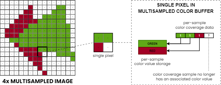
The replacement policy used in these cases may vary across hardware implementations, partly depending on how flexible the mapping supported by the hardware is between color coverage samples and color fragments.
Nonetheless, despite its limitations, keeping the color coverage sample count at full rate while using a reduced number of color storage samples usually results in comparable overall anti-aliasing quality to regular multisampling, while saving precious memory storage and bandwidth, hence the corresponding CSAA and EQAA modes remain popular choices for a wide range of applications.
Bonus: Variable Rate Shading
While technically not a multisampling feature, we need to also mention variable rate shading here.
This feature allows controlling the rate at which fragment shading happens on a per-draw, per-tile, per-viewport, and/or per-primitive basis. Even though the key differentiator of this feature is that it enables shading multiple pixels by a single fragment shader invocation, it also allows controlling the sample shading rate in multisampling use cases.
As such, it provides a way to control the shaded sample count at a granularity that isn’t achievable with traditional sample shading rate parameters. This additional flexibility makes it possible to mix alpha-tested geometry with fully opaque geometry in the same draw call where alpha-tested primitives can use supersampling while the rest of the primitives can still take advantage of the performance benefits of basic multisampling.
Conclusion
In this article we took a look at how increasing spatial sampling frequency at various points in the graphics pipeline enables us to greatly reduce screen-space aliasing and inherently also certain temporal aliasing artifacts (e.g. “travelling” pixels). Supersampling is the most straighforward way to achieve this by uniformly increasing sampling frequency over the entire back-end of the graphics pipeline. We’ve also seen how multisampling attempts to reduce the overhead of supersampling while maintaining most of its quality benefits.
Throughout the article we also presented numerous multisampling features present on modern GPUs that further close the gap between the quality of multisampling and supersampling, including mechanisms that allow us to selectively apply supersampling to certain parts of a scene.
While subject to hardware support, the various advanced multisampling modes can even be combined with one another, enabling fine-grained control over memory/performance/quality trade-offs.
Each individual multisampling feature deserves a much lengthier, in-depth, and more formal description, so this article remains a mere introduction to the topic. Graphics API standard specifications like OpenGL and Vulkan, as well as related extension specifications are likely the best reference out there for rigorous definitions of the behavior of these features. Please, consider the following list of references for further reading:
- OpenGL 4.6 Core Profile Specification
- GL_ARB_multisample (basic multisampling, alpha-to-coverage)
- GL_ARB_sample_shading (sample shading rate)
- GL_ARB_sample_locations (custom sample locations)
- GL_ARB_post_depth_coverage (support for post-depth coverage mask in the fragment shader)
- GL_EXT_raster_multisample (overrasterization)
- GL_AMD_framebuffer_multisample_advanced (separate color coverage and mixed samples rendering)
- GL_NV_framebuffer_multisample_coverage (separate color coverage)
- GL_NV_fragment_coverage_to_color (support to output final coverage mask to a color buffer)
- GL_NV_framebuffer_mixed_samples (mixed samples rendering)
- GL_NV_sample_mask_override_coverage (support to add new lit samples in the fragment shader)
- GL_NV_alpha_to_coverage_dither_control (alpha-to-coverage dithering)
- GL_NV_shading_rate_image (per-tile/viewport variable rate shading)
- GL_NV_primitive_shading_rate (per-primitive variable rate shading)
- Vulkan 1.2 Specification with all published extensions
- VK_KHR_fragment_shading_rate (per-tile/primitive variable rate shading)
- VK_EXT_sample_locations (custom sample locations)
- VK_EXT_post_depth_coverage (support for post-depth coverage mask in the fragment shader)
- VK_EXT_fragment_density_map (per-tile variable rate shading)
- VK_EXT_fragment_density_map2 (per-tile variable rate shading)
- VK_AMD_mixed_attachment_samples (mixed samples rendering)
- VK_AMD_shader_fragment_mask (direct access to color coverage information)
- VK_NV_coverage_reduction_mode (control coverage reduction behavior)
- VK_NV_fragment_coverage_to_color (support to output final coverage mask to a color buffer)
- VK_NV_framebuffer_mixed_samples (mixed samples rendering)
- VK_NV_sample_mask_override_coverage (support to add new lit samples in the fragment shader)
- VK_NV_shading_rate_image (per-tile/viewport variable rate shading)